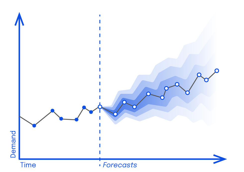
Time Series Data consists of data that involves a time component. For example, the number of sales within a given day, the fluctuating value of a stock, the average temperature in a specific region, etc.

They can have continuous or discrete values and exhibit a wide range of behavior over time:

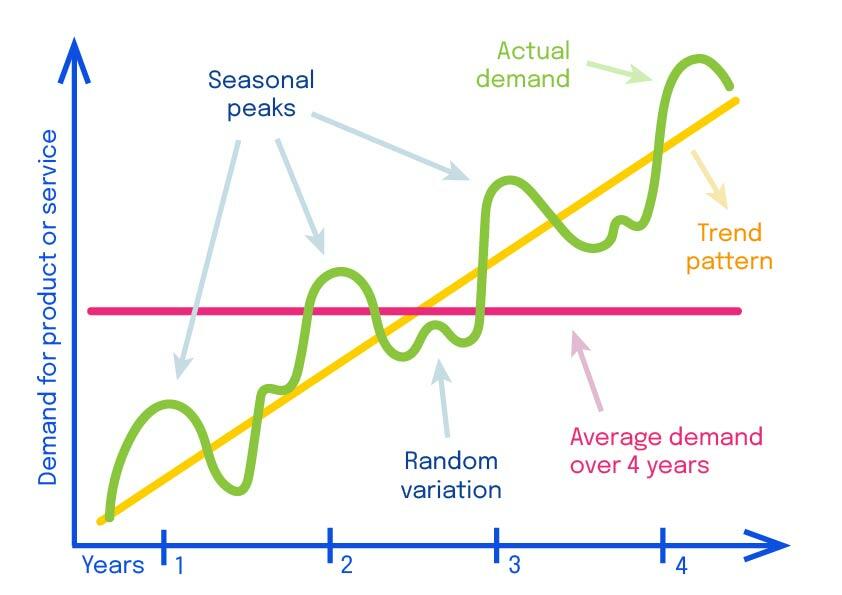
• Trends are long-term patterns going in the same overall direction;
• Cycles are non-periodic repetitive patterns, such as highs and lows of the stock market, where the time intervals between the highs and the lows is variable;
• On the other hand, seasonality is a pattern that repeats periodically (think of higher demand for gift wrap around Christmas for instance);
• Lastly, responses to outside stimuli and random events are possible factors that drive the time evolution of a given quantity. Noise and sparseness make it challenging to extract a signal and make predictions.

In addition, time series are often co-dependent and therefore need to be considered together. A typical scenario is where one time series (a covariate) is used to inform predictions about another (the response or observation). For example, a time series representing whether a day is or isn’t a holiday can be used as a covariate (a.k.a. a feature) for making predictions of daily sales.

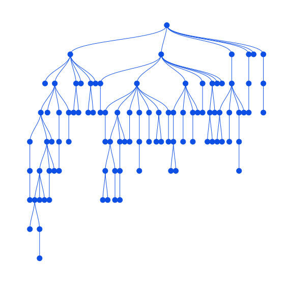
Furthermore, in most real-world cases, multiple time series exist in a hierarchical structure (hierarchical time series). For example, the sales numbers of different products can be aggregated into product categories, or regional sales can be aggregated into national sales.

The number of individual time series across the whole structure may be very large. Since they are also typically sparse and noisy at the most granular level, aggregating them allows for more regular results and more accessible analysis.

(Automatic) Forecasting is hard

Time series are very useful when trying to understand the historical development of a given domain. Some of the most common questions are: how will my product or service develop in the future? Will the trend continue? Are the seasonal patterns dependable? And how certain are we about these things?

It would be nice to always have a statistician or a time series expert on hand to answer these types of questions… but you can probably guess that it is not very practical and can get quite expensive.

Automatic forecasting systems therefore exist to provide reasonable forecasts even in the hands of non-experts.

To give an automated answer to the questions above, while keeping we need the system to produce probabilistic forecasts. This means that the forecast does not only consist of a single value that could be off (which is the method historically used), but of a distribution of values that keeps into account an estimate of the uncertainty (which represents the probability of having a true number within a range of values). When appropriately visualized, this allows non-experts to assess the forecast.

A good graph can give anyone a quick sense of the range of possible outcomes and their respective probabilities

Yet, despite the apparent simplicity of an automatically generated graph, making automatic probabilistic forecasts work robustly across many use cases is very hard. The complexity and variety of time series (temporal patterns, variety of data types, noise, hierarchical structures of different kinds, length, and quantity of time series) create a big challenge.

Without the uncertainty adjustments, we don’t really know how trustworthy the forecast is.

In addition, forecasts for hierarchical time series should be developed in a way that is coherent. For example, forecasts of aggregated sales should match the aggregation of the forecasts of individual sales.

Forecasting for hierarchical time series usually proceeds in two steps:

1. First, forecasts are made for each individual time series,
2. In the second step, called reconciliation, these forecasts are adjusted with the appropriate probabilistic methods to become coherent. In this process, the uncertainty estimates of individual series are also combined in a meaningful way for the reconciled forecasts.

Here’s a visual example of how reconciliation works:

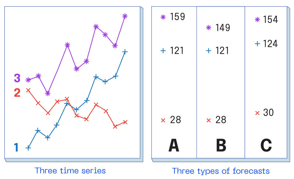
In the left figure, you can see the development of three time series: 1 (blue) and 2 (red) which represent collected historical data, and 3 (purple) which is their sum.

In the right figure, we find three types of forecasts:

• A, shows the so-called “base forecasts”, which are predictions of each time series considered individually, and it doesn’t take into account the fact that 3 is a sum of the others.
• B, shows “bottom-up forecasts”, which differ from “base forecasts” because here we do take into account that 3 is a sum of time series 1 + 2 (ie. 28 + 121 = 149). This type of forecast is technically coherent, but it is problematic because it places unmerited certainty on the forecasts of 1 and 2. It also doesn’t take the purple data (time series 3) into account.
• C, is the type of forecast we aim at, where the three predictions produce a coherent result in which all three base forecasts are adjusted according to their uncertainty. Taking uncertainty into consideration means we can make a forecast that is more likely to match the real outcome (generally aiming at 90–95% accuracy in the prediction).

As with the models for individual time series, the reconciliation method should be robust across a wide range of time series types and ideally allow for many types of interdependence.

In summary, developing an automated forecasting solution that addresses all these different challenges is not straightforward.

Once past this problem, however, the ensuing customized automatic forecasts can be integrated into a workflow that can be leveraged by decision makers.

Combining Gaussian Processes and Probabilistic Reconciliation for Automatic Forecasting

At this stage, you might be thinking: how do we overcome this problem?

Gaussian processes (GPs) are very flexible models that define the distribution between variables in time and space. When combined with a probabilistic reconciliation method, they solve all of the above-mentioned challenges almost out of the box.

GPs are naturally probabilistic, as they model a complete distribution over possible ways a time series can evolve. This so-called Gaussian distribution shows the correlation of observations at different points in time: this allows us to capture a wide range of temporal behaviors. The temporal patterns described by GPs offer templates that can be tuned to a particular time series in order to make forecasts.

The various ranges predicted can then be narrowed down to smaller ranges with each new data point. Imagine that the GP already has a notion of the different trajectories that a time series might take, but each additional data point narrows that down to trajectories that are likely to have occurred.

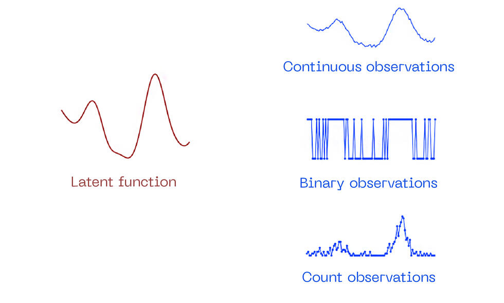
Additionally, in the second stage, we can generate different distributions of the collected data by using the GP to model a latent function that is not observed directly, but via another random process.

This two-stage model with non-Gaussian observations can be used to describe a wider range of data that was previously unrecognized and make better forecasts.

Of course, all that flexibility and power do not come easily. In order to apply GPs in practice, a number of technical difficulties need to be overcome:

• First of all, since each individual time series is different, a single GP model cannot be applied to all of them. Therefore, appropriate parameter settings have to be found for each time series individually;
• Non-Gaussian observations also make the model much more difficult to handle, because approximations need to be used to make it more manageable;
• In their most basic form, GPs scale poorly to larger datasets because of their cubic complexity in the number of observations, which greatly increases the algorithm’s processing time.

These issues have stood in the way of the widespread adoption of GPs as time series models, especially in automatic forecasting contexts.

Luckily, recent advances have changed this.

State-of-the-art approximation techniques, automatic differentiation, and the use of GPU hardware allow GPs to be efficiently trained on larger datasets and with non-Gaussian observations.

Thanks to these latest innovations, automatic forecasting systems have become more precise and reliable than ever before. This means you can find answers to your what if ’s with better predictions and make more informed decisions for your business’ success.